Statistics
Exploring Predictive factors for Heart Disease: A Comprehensive Analysis Using Logistic Regression
Fall 2024, Volume 23, Issue 1
Haolin Wang ’25, Aruni Jayathilaka*
https://doi.org/10.47761/YRCU1073
Introduction
Heart disease is a significant issue in the global health field. In the US, more than 690,000 people die of heart disease each year and more than 800,000 people will experience a heart attack. Thus, understanding predictive factors is crucial for effective prevention and diagnosis [6]. In this study, we analyze a comprehensive dataset relating to heart disease from UCI Machine Learning Repository [8]. It comprises records from four databases collected from Cleveland, Hungary, Switzerland, and the Veterans Affair (VA) Long Beach. It includes 13 features, focusing on attributes such as age, sex, chest pain type, and cholesterol levels, among others. These features are divided into two types: categorical and integer. Logistic regression is used to explore the impact of various factors on heart disease. The methods include data preprocessing, model selection using Akaike Information Criterion (AIC), and model interpretation.
In developing a logistic regression model to predict heart disease, our approach aligns with Zhang, Diao, and Ma, who demonstrated logistic regression’s effectiveness in heart disease prediction among the elderly, emphasizing the model’s potential in clinical settings [5]. Furthermore, our findings cohered with those of Anshori and Haris, who demonstrated logistic regression’s high accuracy in diagnosing heart disease using comprehensive patient medical records [4]. Beyond heart disease, logistic regression has been effectively applied in other medical fields. For example, Nusinovici compared logistic regression with machine learning algorithms in predicting chronic diseases such as diabetes and hypertension, showing that logistic regression often performs well [3]. These references collectively reinforce the applicability and efficacy of logistic regression models in the field of medical prediction and diagnostics, providing a strong foundation for our study.
The article identifies some key features related to heart disease, including sex, maximum heart rate (HR), type of chest pain, blood pressure, cholesterol level, the number of vessels shown in coronary angiography, ST depression, and slopes of ST and Thallium were identified as key factors that significantly influence heart disease occurrence. The logistic regression model constructed through a backward elimination approach allowed us to quantify the relative impact of each variable on the probability of heart disease.
In the model evaluation section, we introduced the AIC as a powerful tool for model selection, balancing goodness of fit and model complexity [7]. Furthermore, the concept of the confusion matrix was explained, along with the calculation of metrics such as accuracy and precision [1]. These metrics comprehensively assessed the performance of the logistic regression model in predicting heart disease.
1. Logistic Regression
1.1: Introduction to the Binary Logistic Regression Model
Logistic regression is a powerful statistical learning model used for binary classification problems. Fundamentally, the model maps the output of a linear regression model through a logistic function, transforming predictive values into probability values. These are then used to make classification decisions [1]. Here, we introduce the core concepts of logistic regression, including the model’s definition and its basic assumptions, and we will derive the estimation process of the model parameters in detail using the maximum likelihood estimation method.
Definition of Logistic Regression:
Logistic regression is a statistical model used to depict the probability of a binary outcome, often coded as 0 or 1, based on one or more predictor variables. The main goal of logistic regression is to determine the likelihood that a particular event will occur, as a function of the input variables. The probability that an event occurs, represented as P (Y = 1), is given by the formula:
- P(Y = 1) is the probability of the event occurring. e is the base of the natural logarithm.
- β0, β1, . . . , βk are the coefficients of the model, indicating the impact of each input variable on the probability of the event occurring.
- X1, X2, . . . , Xk are the values of the input variables.
Derivation of Maximum Likelihood Estimation:
To estimate the parameters of the logistic regression model, this paper uses the maximum likelihood estimation method [1]. The objective of maximum likelihood estimation is to find a set of parameters that maximize the likelihood function for the observed sample data. For logistic regression, the likelihood function is:
- N is the number of samples.
- Yi is the actual category of the ith observed sample (0 or 1).
- yi is the probability of the predicted category for the ith sample, given by the logistic regression model.
- P(Yi = yi) is the predicted probability that the outcome Yi is equal to yi.
The goal of the likelihood function is to maximize this probability, or more specifically, to find the model parameters β0, β1, . . . , βk, that make the probability of observing the data the highest. Usually, for the convenience in calculation, the natural logarithm of the likelihood function is taken, resulting in the log-likelihood function:
 Logistic regression usually uses an iterative method (such as gradient descent) to initiate maximum likelihood estimation to obtain the coefficients of the model.
2. Interpretation of the Fitted Logistic Regression Model
2.1: Akaike Information Criterion (AIC)
The AIC is a statistical criterion for model selection, proposed by the Japanese statistician Hirotugu Akaike. The core idea of AIC is to balance the evaluation of model fit and complexity. It considers the fit of the model to the data and complexity of the model to avoid overfitting. The formula for calculating AIC:
AIC = 2 × log-likelihood + 2 × number of parameters
Here, the log-likelihood is the value of the log-likelihood function for the model fitted to the observed data, and the number of parameters is the count of parameters in the model. The goal of AIC is to minimize its value, as it takes into account both the goodness of fit of the model and its complexity.
2.2: Confusion Matrix and Accuracy
The confusion matrix is a table used to evaluate the performance of models, particularly suitable for binary classification problems. Through the confusion matrix, we can calculate the following metrics:


3. Dataset
3.1: Summary of the Dataset
This study uses a dataset on heart disease to investigate factors associated with the risk of heart disease. The dataset contains multiple key variables, which are believed to be potentially related to the occurrence of heart disease.
Variable Definition:
- Sex: Represents the individual’s biological sex, categorized as male or female (0: female, 1: male).
- Age: Records the age information of each individual (29 – 77 years).
- Chest Pain Type: Describes the type of angina pectoris (1: typical angina, 2: atypical angina, 3: non-anginal pain, 4: asymptomatic).
- Blood Pressure (BP): Measures the individual’s blood pressure level (94 – 200 mmHg).
- Cholesterol Level: Records the individual’s cholesterol level (126 – 564 mg/dl).
- Fasting Blood Sugar (FBS): Indicates whether the individual’s blood sugar level exceeds 120 mg/dl when fasting (0: No, 1: Yes).
- EKG Results: Describes the findings of the electrocardiogram, (0: normal, 1: ST-T wave abnormality, 2: probable or definite left ventricular hypertrophy).
- Maximum Heart Rate (Max HR): Records the maximum heart rate achieved by the individual (71 – 202 beats/minute).
- Exercise Angina: Indicates whether the individual experiences angina during exercise (0: No, 1: Yes).
- ST Depression: Measures the level of ST segment depression (0 – 6.2).
- Slope of ST: Describes the slope characteristics of the ST segment (1: up-sloping, 2: flat, 3: down-sloping).
- Number of Vessels in angiography: Records the number of vessels shown in coronary angiography (0 – 3).
- Thallium Test Results: Describes the results of the Thallium test (3: normal, 6: fixed defect, 7: reversible defect).
- Heart Disease: Whether a person has heart disease (0: No, 1: Yes).
Through the analysis of these variables, this paper aims to establish a model for predicting the probability of heart disease occurrence, to gain a deeper understanding of the impact of various factors on the risk of heart disease.
3.2: Data Visualization
1. Age and the occurrence of heart disease: (Fig.1)
Visualization results: The boxplot of age versus the occurrence of heart disease shows that the median, first, and third quartile of individuals with heart disease are higher than individuals without heart disease, and individuals with heart disease exhibit a left-skewed distribution.
Statistical results: The average age of individuals without heart disease is 52.7, with a median age of 52; for individuals with heart disease, the average age is 56.6, with a median age of 58. Based on the results above, it suggests that older people might have a higher chance to gain heart disease.
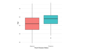 Figure 1: Boxplot of Age Distribution
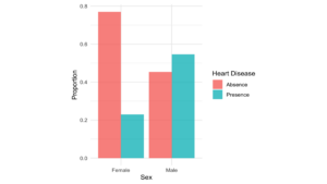 Figure 2: Sex Barplot
2. Sex and the occurrence of heart disease: (Fig.2)
Visualization results: The bar chart of sex versus the occurrence of heart disease shows that there are more cases of heart disease among males than females.
Statistical results: The probability of males having heart disease in our sample is 54.64%, compared to females (22.99%).
3. Chest pain type and the occurrence of heart disease: (Fig.3)
Visualization results: The bar chart of chest pain type versus the occurrence of heart disease shows that among individuals with chest pain type 4(asymptomatic), the rate of having heart disease is apparently higher than the other three types.
Statistical results: The probability of heart disease cases with chest pain type 4 is 70.54%, compared to other three types (25.00%, 16.67%, 21.52%).
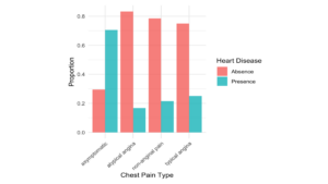 Figure 3: Chest Pain Type Barplot
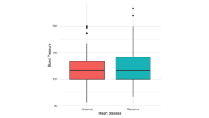 Figure 4: Boxplot of Blood Pressure
4. Blood pressure and the occurrence of heart disease: (Fig.4)
Visualization results: The boxplot of blood pressure versus the occurrence of heart disease shows that there is no significant difference between individuals with and without heart disease.
Statistical results: The average blood pressure of individuals without heart disease is 128.87, with a median age of 130; for individuals with heart disease, the average age is 134.442, with a median age of 130. Based on the results above, it suggests that blood pressure might have no impact on the occurrence of heart disease.
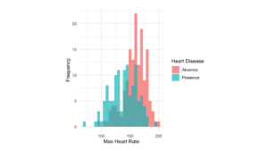 Figure 5: Max Heart Rate Distribution Plot
5. Maximum heart rate and the occurrence of heart disease: (Fig.5)
Visualization results: The histogram of maximum heart rate versus the occurrence of heart disease shows that individuals with heart disease tend to have a relatively lower maximum heart rate.
Statistical results: The average maximum heart rate for individuals without heart disease is 158, with a median of 161; for individuals with heart disease, the average maximum heart rate is 139, with a median of 142.
4. Model Selection
4.1: Exploring the Full Model
In the process of fitting the full model, this paper adopts a binary logistic regression model, aiming to gain a deeper understanding of the characteristics of the heart disease dataset. The full model includes multiple predictive variables, among sex, age, chest pain type, and other key factors. This section will detail the steps of fitting the full model, model selection by backward elimination, and various aspects of reduced model.
4.2: Binary Logistic Regression Model
First, the paper reviews the definition and basic assumptions of the binary logistic regression model. The logistic regression model is a statistical learning model for binary classification problems, used to predict the probability of occurrence of a certain event. The basic form of the model is as follows:
- p is the probability of the presence of the characteristic of interest (e.g. having heart disease).
- p is the odds ratio (OR) of the characteristic of interest occurring or not. Xj represents the independent variables (predictors).
- βk represents the coefficients that measure the impact of predictors.
Table 1 Logistic Regression Coefficient Summary
| coefficients | ||||
| estimate | std. error | z value | p value | |
| (intercept) | -6.970 | 3.150 | -2.213 | 0.027 |
| Male | 1.763 | 0.581 | 3.036 | 0.002 |
| Age | -0.016 | 0.026 | -0.606 | 0.544 |
| Atypical Angina | 1.389 | 0.893 | 1.555 | 0.119 |
| Non-Anginal Pain | 0.553 | 0.747 | 0.739 | 0.459 |
| Asymptomatic | 2.386 | 0.757 | 3.154 | 0.002 |
| Blood Pressure | 0.026 | 0.012 | 2.153 | 0.032 |
| Cholesterol | 0.007 | 0.004 | 1.566 | 0.117 |
| Fasting Blood Sugar | -0.370 | 0.626 | -0.591 | 0.555 |
| EKG.abnormality | 0.648 | 3.185 | 0.203 | 0.839 |
| EKG.left ventricular hypertrophy | 0.634 | 0.412 | 1.538 | 0.124 |
| Max.HR | -0.019 | 0.011 | -1.683 | 0.092 |
| Exercise.angina | 0.597 | 0.461 | 1.296 | 0.195 |
| ST.depression | 0.449 | 0.245 | 1.836 | 0.06 |
| Flat ST | 0.950 | 0.500 | 1.898 | 0.058 |
| Down-sloping ST | 0.123 | 1.042 | 0.118 | 0.906 |
| Number of Vessels | 1.200 | 0.281 | 4.271 | 0.000 |
| Thallium.fixed | -0.146 | 0.846 | -0.173 | 0.863 |
| Thallium.reversible | 1.432 | 0.450 | 3.183 | 0.001 |
4.3: Model Generated by Backward Selection
Method of Backward Selection:
For the model selection process, this paper uses the method of backward selection, evaluating the model’s performance through the Akaike Information Criterion (AIC). Backward selection improves the model’s simplicity by progressively eliminating variables that contribute less to the model.
Model Selection Results:
The results of backward elimination show that the final model includes key variables such as sex, chest pain type, blood pressure (BP), cholesterol level, max heart rate, ST.depression, slope of ST, number of vessels shown in coronary angiography and thallium. These variables are considered to have a significant impact on the occurrence of heart disease.
Table 2 Backward Regression Coefficient Summary
| coefficients | ||||
| estimate | std. error | z-value | p-value | |
| (intercept) | -7.193 | 2.648 | -2.717 | 0.007 |
| Male | 1.851 | 0.562 | 3.295 | 0.001 |
| Atypical Angina | 1.264 | 0.883 | 1.432 | 0.152 |
| Non-Anginal Pain | 0.446 | 0.748 | 0.596 | 0.551 |
| Asymptomatic | 2.532 | 0.749 | 3.381 | 0.001 |
| Blood Pressure | 0.024 | 0.011 | 2.178 | 0.029 |
| Cholesterol | 0.007 | 0.004 | 1.812 | 0.070 |
| Max.HR | -0.020 | 0.011 | -1.925 | 0.054 |
| ST.depression | 0.467 | 0.233 | 2.002 | 0.045 |
| Flat ST | 1.025 | 0.493 | 2.078 | 0.038 |
| Down-sloping ST | 0.166 | 0.991 | 0.167 | 0.867 |
| Number of Vessels | 1.135 | 0.262 | 4.338 | 0.000 |
| Thallium.fixed | -0.324 | 0.813 | -0.398 | 0.691 |
| Thallium.reversible | 1.377 | 0.428 | 3.215 | 0.001 |
4.4: Model Analysis
Using the glm function in R, this paper successfully fitted a binary logistic regression model. The fitting results of the model are displayed using the summary function, which includes the coefficients, standard errors, z-values, p-values, etc., for each predictive variable. This paper focuses on the significance of each coefficient to determine whether the variables have a statistically significant impact on the occurrence of events.
Furthermore, the paper conducted model diagnostics, including using the Box-Tidwell test to check the model’s linearity, the Durbin-Watson test to verify the independence of observations, VIF to examine multicollinearity, and MC distance to check the extreme outliers. This series of diagnostic processes helps to ensure the model’s reasonableness and accuracy.
Assumption:
- Multicollinearity checking: VIF (Variance Inflation Factor) values are used to test for multicollinearity, and most variables have VIF values within a reasonable range (less than 2), suggesting that the influence of multicollinearity among variables is minimal. Since no VIF value exceeds 2, the multicollinearity may not be considered as an issue.
- Independence checking: The Durbin-Watson statistic is 2.137, with a p-value of 0.262. The statistic being close to 2 and the relatively large p-value suggest that there is no significant auto-correlation between different variables, indicating that the variables are independent.
- Linearity checking: Check the linearity of logistic regression by Box-Tidwell. The Box-Tidwell test is for checking the linearity between continuous predictors and the logit of the dependent variable. The significance of Box-Tidwell means the non-linear relationship between predictors and the logit of the dependent variable. From the result of the Box-Tidwell test, we can find out that the p-value of all continuous variables is larger than 0.05, which indicates no violation of linearity needs to be considered.
- Outliers checking by Cook’s distance: By calculating Cook’s Distance, it is possible to identify outliers that may have a significant impact on the model. Based on the plot, potential outliers can be identified – those whose Cook’s Distance exceeds a predetermined threshold – and these outlier points can be removed. Although some observations’ Cook’s Distance might be much higher than other points (2, 88, and 265), they can not be considered as influential points since their Cook’s Distances are all less than 0.5, indicating that they do not have significant impacts on the model results after removing them.
4.5: Model Explanation
Influence of Parameters:
By interpreting the model parameters, this paper focuses on the relative contributions of various variables to the probability of occurrence of heart disease, holding all other variables constant. In logistic regression, the coefficients represent the change in the log odds of the outcome for a one-unit increase in the predictor variable or different types, with all other variables held constant. Exponentiate coefficient for translating the coefficient into an odds ratio. If the coefficient is positive, indicating that the odds of having heart disease will time some value (exp(coefficient)) higher than 1, which will raise the occurrence of heart disease, in contrast, the negative coefficient will decrease the occurrence of heart disease.
- Sex: When a patient’s sex is male, the odds of a patient having heart disease are exp(1.851) = 6.366 times the odds of a female patient having heart disease, holding all other variables constant.
- Chest Pain Type: When a patient’s chest pain type is Atypical Angina, Non-Anginal Pain and Asymptomatic, the odds of a patient having heart disease are exp(1.264) = 3.540, exp(0.446) = 1.562, exp(2.532) = 12.579 times the odds of patient’s chest pain type is typical angina, holding all other variables constant.
- Blood Pressure (BP): For each 1 mmHg increase in the patient’s Blood Pressure, the odds of having heart disease multiply by exp(0.024) = 1.024, holding all other variables constant.
- Number of Vessels Shown in Coronary Angiography: For each number increase in patient’s vessels shown in Coronary Angiography, the odds of having heart disease multiply by exp(1.1346) = 3.110, holding all other variables constant.
- ST depression: For each 1 unit increase in ST segment depression, the odds of having heart disease multiply by exp(0.467) = 1.595, holding all other variables constant.
- Slopes of ST: When a patient’s slope of ST is flat and down-sloping, the odds of a patient having heart disease are exp(1.025) = 2.787, exp(0.166) = 1.181 times the odds of the patient’s slope of ST is up-sloping, holding all other variables constant.
- Thallium: When a patient’s thallium test result is a fixed defect and reversible defect, the odds of a patient having heart disease are exp(−0.324) = 0.723, exp(1.377) = 3.963 times the odds of the patient’s thallium test result is normal, holding all other variables constant.
- Cholesterol: For each 1 mg/dl increase in the patient’s cholesterol level, the odds of having heart disease multiply by exp(0.007) = 1.007, holding all other variables constant.
- Max.HR: For each 1 unit of heart rate increase for patients, the odds of having heart disease multiply by exp(−0.020) = 0.980, holding all other variables constant.
Overall Performance
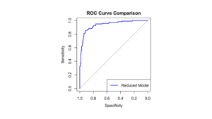 Figure 6: ROC Curve
The overall performance of the Backward reduced model is evaluated using a confusion matrix and ROC curve (Fig.6). An ROC curve with an AUC of 0.8692 indicates that the model has a high accuracy in predicting heart disease. The model’s accuracy is 87.41%, and the confusion matrix shows the model’s predictive performance.
Confusion Matrix of Reduced Model:
| Predicted | |||
| 0 | 1 | ||
| True | 0 | 137 | 13 |
| 1 | 21 | 99 |
Likelihood Ratio Test:
Comparing the reduced model with the full model, by using the Likelihood Ratio Test (LRT) for model comparison. The full model (Model 1) includes all predictor variables, while the backward regression model (Model 2) achieves model simplification by gradually removing some variables. During the model comparison process, differences between Model 1 and Model 2 were observed and the corresponding p-value was calculated. The results show that the reduced model is adequate (p-value = 0.457), indicating that the additional variables in Model 1 might not provide sufficient explanatory power and the simpler Model 2 is, the more preferable due to its parsimony.
Conclusion
In summary, our research comprehensively analyzed the predictive factors for heart disease using logistic regression. Through a rigorous process of model selection and validation, we successfully reduced the variables from 13 to 9, and identified key variables such as sex, max. HR, cholesterol, type of chest pain, blood pressure, number of vessels, ST slopes, ST depression, and Thallium levels as significant predictors for the occurrence of heart disease. The logistic regression model, selected based on the AIC, provides a quantifiable understanding of each variable’s influence on heart disease risk.
This study’s findings underscore the importance of these predictors in clinical settings, offering healthcare professionals a robust tool for early identification and management of individuals at high risk for heart disease. The model’s high accuracy (0.874), as evidenced by the ROC curve and confusion matrix, demonstrates its potential utility in real-world applications, particularly in preventative health strategies and personalized medicine.
Furthermore, assumption checks for multicollinearity, independence, linearity, and outliers confirmed the model’s reliability, ensuring that the results are both statistically and clinically valid. Data visualization techniques were used to enhance the interpretability of key variables, providing clear insights into their relationship with heart disease occurrence.
However, this research is not without limitations. The dataset used, although comprehensive, may not capture all potential risk factors for heart disease. Future research could benefit from incorporating additional variables such as genetic markers, lifestyle factors, and other biomarkers to improve the model’s predictive power. Additionally, the model’s applicability to diverse populations needs further investigation to ensure its generalizability across different demographic groups. Furthermore, we acknowledge that the dataset used in this study is relatively dated and may not fully capture the current trends and patterns in heart disease risk factors. To enhance the relevance and accuracy of future predictions, it would be beneficial to utilize updated datasets, potentially sourced from electronic medical records (EMRs) and other modern data collection techniques. Access to current data would allow for the identification of contemporary risk factors that are more reflective of the present-day patient population, thereby improving the model’s applicability and accuracy.
Overall, this research provides a valuable meaning for understanding the predictive factors of heart disease, offering significant implications for both clinical practice and public health strategies and contributing to the ongoing fight against heart disease on a global scale.
References
- Hosmer, David W., et al. Applied Logistic Regression David W. Hosmer, Stanley Lemeshow, Rodney X. Sturdivant. 3rd ed., Wiley, 2013.
- Zach, Bobbitt. The 6 Assumptions of Logistic Regression (with Examples). Statology, 13 Oct. 2020, www.statology.org/assumptions-of-logistic-regression/
- S. Nusinovici et al. Logistic regression was as good as machine learning for predicting major chronic diseases. Journal of Clinical Epidemiology (2020). https://doi.org/10.1016/j. jclinepi.2020.03.002
- M. Anshori et al. Predicting Heart Disease using Logistic Regression. Knowl. Eng. Data Sci., 5 (2022): 188-196. https://doi.org/10.17977/um018v5i22022p188-196
- Yingjie Zhang et al. Logistic Regression Models in Predicting Heart Disease. Journal of Physics: Conference Series, 1769 (2021). https://doi.org/10.1088/1742-6596/1769/1/012024
- J. Cavanaugh et al. The Akaike information criterion: Background, derivation, properties, application, interpretation, and refinements. Wiley Interdisciplinary Reviews: Computational Statistics, 11 (2019). https://doi.org/10.1002/wics.1460.
- Janosi, A., Steinbrunn, W., Pfisterer, M., & Detrano, R. (1989). Heart Disease [Dataset]. UCI Machine Learning Repository. https://doi.org/10.24432/C52P4X.
About the Author
My name is Haolin Wang, a senior student major in statistics and business information system. My interest is merging statistics with healthcare, channeling my analytical expertise and entrepreneurial spirit to develop innovative solutions for chronic patient care and early disease detection. I have develop a smoke cessation app and Antibiotic- Resistant bacterial Strain database. My scientific interest is using of advanced statistical model to creating a smart wristband to avoid stroke patients miss the critical window from onset to treatment.
Cite this Article
Wang, H. and Jayathilaka, A. (2024). Exploring Predictive factors for Heart Disease: A Comprehensive Analysis Using Logistic Regression. University of Rochester, Journal of Undergraduate Research, 23(1). https://doi.org/10.47761/YRCU1073
JUR | Creative Commons Attribution 4.0 BY International License